| Table of Contents |
|---|
Introduction
...
For a set of zones z = {1, 2, 3, ..} the relative illumination of zone n is 2-(z-1) = {1, 0.5, 0.25, 0.125, …}. The illumination difference between zones is {0.5, 0.25, 0.125, …}. The scene illumination ratio between zones is always 2:1.
| Tip |
|---|
Geek alert: a lot of numbers follow— all of which are intended to show how gamma encoding increases the effective dynamic range. The total number of available pixel levels B is a function of the bit depth, B = 2(bit depth). For bit depth = 8, B = 256; for bit depth = 16, B = 65536. The relative pixel level of zone n for encoding gamma γe is bn = B × 2-(n-1)γe. For linear gamma (γe = 1), bn= {1.0, 0.5, 0.25, 0.125, …} (the same as L). For γe= 1/2.2 = 0.4545, bn = {1.0000, 0.7297, 0.5325, 0.3886, 0.2836, 0.2069, 0.1510 ,0.1102, …}. The relative pixel levels bn decrease much more slowly than for γe = 1. The relative number of pixel levels in each zone is npγ(i) = bn(i) – bn(i+1), which brings us to the heart of the issue. For a maximum pixel level of 2(bit depth)-1 = 255 for widely-used files with bit depth = 8 (24-bit color), the total number of pixels in each zone is Npγ(i) = 2(bit depth)npγ(i). |
...
...
| Tip |
|---|
For linear images (γe = 1), npγ(i) = {0.5, 0.25, 0.125, 0.0625, …}, i.e., half the pixel levels would be in the first zone, a quarter would be in the second zone, etc. For files with bit depth = 8, the zones starting from the brightest would have Npγ(i) = {128, 64, 32, 16, 8, 4, 2, 1 …} pixel levels of 256 (0-255). By the time you reached the 5th or 6th zone, the spacing between pixel levels would be small enough to cause significant “banding”, limiting the dynamic range. For images encoded with γe = 1/2.2 = 0.4545, the relative number of pixels in each zone would be bn(i) = {0.2703, 0.1972, 0.1439, 0.1050, 0.0766, 0.0559, 0.0408, 0.0298, 0.0217, 0.0159…}, and the total number Npγ(i) would be {69.2, 50.5, 36.8, 26.9, 19.6, 14.3, 10.4, 7.63, 5.56, 4.06, …} of 256. The sixth zone, which has only 4 levels for γe = 1, has 14.3 levels. The 10th gamma-encoded zone has the same number of levels (4) as the 6th linear zone, i.e., an effective dynamic range increase of up to four zones (f-stops; factors of 2). To summarize: |
| Info |
These numbers show how gamma-encoding greatly improves the effective dynamic range of images with limited bit depth by redistributing pixel levels so there are more in darker zones and fewer in lighter zones (which have way more than needed in linear systems). Of course, the improvement will be less if flare light in dark regions is the limiting factor. |
What gamma (and Tonal Response Curve) should I expect?
And what is good?
...
A brief history of chart contrast 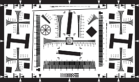 The ISO 12233:2000 standard called for a chart contrast of at least 50:1. This turned out to be a poor choice: The high contrast made it difficult to avoid clipping (flattening of the tonal response curve for either the lightest or darkest areas), which exaggerates MTF measurements (making them look better than reality). There is no way to calculate gamma from the ISO 12233:2000 chart (shown on the right). This issue was finally corrected with ISO 12233:2014 (later revisions are relatively minor), which specifies a 4:1 edge contrast, which not only reduces the likelihood of clipping, but also makes the MTF calculation less sensitive to the value of gamma used for linearization. The old ISO 12233:2000 chart is still widely used: we don’t recommend it.  The SFRplus chart, which was introduced in 2009, originally had an edge contrast of 10:1 (often with a small number of 2:1 edges). After 2014 the standard contrast was changed to 4:1 (shown on the right). The eSFR ISO chart (derived from the 2014 standard) always has 4:1 edge contrast. Both SFRplus and eSFR ISO have grayscales for calculating tonal response and gamma. SFRreg and Checkerboard charts are available in 10:1 and 4:1 contrast. Advantages of the new charts are detailed here and here. Imatest chrome-on-glass (CoG) charts have a 10:1 contrast ratio: the lowest that can be manufactured with CoG technology. Most other CoG charts have very high contrast (1000:1, and not well-controlled). We don’t recommend them. We can produce custom CoG charts quickly if needed. |
...
We ran an image from a compact digital camera, converted from raw with dcraw, with a number of different gamma settings to see how the settings affected MTF rsults.
...
Tonal response from grayscale. gamma = 0.369
...
The chart and images are several years old. The chart may have been printed with lower contrast than intended, resulting in a lower gamma measurement. This has no effect on the relative measurements below
...
Gamma | MTF50 (C/P) | MTF Area PkNorm (C/P) |
0.20 | 0.2415 | 0.261 |
0.30 | 0.2408 | 0.258 |
0.322 | 0.2368 | 0.254 |
0.40 | 0.2387 | 0.254 |
0.50 | 0.2344 | 0.247 |
0.60 | 0.2332 | 0.247 |
...
JPEGs, on the other hand, frequently have a “shoulder”— a region where gamma (contrast) is gradually reduced— in the highlights. The shoulder improves the perceived pictorial quality of the image by reducing saturation (or “burnout”) of the highlights. It was a part of film response curves, long taken for granted. In order to achieve this shoulder, the exposure has to be reduced below the optimum level for a straight gamma curve to allow some “headroom” for the shoulder (before highlights are saturated). Here is an example: in-camera JPEG and LibRaw-converted raw images of the Colorchecker charts and doll, whose tonal response curve are shown above or the in-camera JPEG and below for the LibRaw-converted TIFF.
  |   |
Here is the (nearly) straight-line density response for the converted CR2 raw image on the right. Though this image is typical, we have seen much larger differences between JPEG and converted raw files.
...
| Eazy math inline | ||
|---|---|---|
|
...
If we assume that exp is normalized to a maximum value of expmax = 1, p(expmax) = p(1) = 1. The darkest level that can be reproduced is p(expmin) = γ log10(expmin)+1 = 0.
| Eazy math inline | ||
|---|---|---|
|
...
For gamma = 0.5 (shown in the plot, above right), expmin = 10-2 = 0.01, equivalent to
| Eazy math inline | ||
|---|---|---|
|
| Eazy math inline | ||
|---|---|---|
|
...
The chart on the right is designed for a visual measurement of display gamma. But it rarely displays correctly in web browsers (and may never display correctly on this Atlassian page, where there is no way to set it to 100% size). It has to be displayed in the monitor’s native resolution, 1 monitor pixel to 1 image pixel. Unfortunately, operating system scaling settings and browser magnifications can make it difficult.  |
|

To view the gamma chart (on the right) correctly, right-click on it, copy it, then paste it into Fast Stone Image Viewer.
This worked well for me on my fussy system where the main laptop monitor and my ASUS monitor (used for these tests) have different scale factors (125% and 100%, respectively).
The gamma will be the value on the scale where the gray area of the chart has an even visual density. For the (blurred) example on the left, gamma = 2.
Although a full monitor calibration (which requires a spectrophotometer) is recommended for serious imaging work, good results can be obtained by adjusting the monitor gamma to the correct value. We won’t discuss the process in detail, except to note that we have had good luck with Windows systems using QuickGamma.
...

Appendix II: Tonal response, gamma, and related quantities
For completeness, we’ve updated and kept this table from elsewhere on the (challenging to navigate) Imatest website.
Parameter | Definition | ||||||||||||||||||||
Tonal response curve | The pixel response of a camera as a function of exposure. Usually expressed graphically as log pixel level vs. log exposure. | ||||||||||||||||||||
Gamma | Gamma is the average slope of log pixel levels as a function of log exposure for light through dark gray tones). For MTF calculations It is used to linearize the input data, i.e., to remove the gamma encoding applied by image processing so that MTF can be correctly calculated (using a Fourier transformation for slanted-edges, which requires a linear signal). Gamma defaults to 0.5 = 1/2, which is typical of digital camera color spaces, but may be affected by image processing (including camera or RAW converter settings) and by flare light. Small errors in gamma have little effect on MTF measurements for 4:1 (low) contrast ratio edges (See How strongly does gamma affect MTF? above). Gamma should be set to 0.45 or 0.5 when dcraw or LibRaw is used to convert RAW images into sRGB or a gamma=2.2 (Adobe RGB) color space. It is typically around 1 for converted raw images that haven’t had a gamma curve applied. If gamma is set to less than 0.3 or greater than 0.8, the background will be changed to pink to indicate an unusual (possibly erroneous) selection. If the chart contrast is known and is ≤10:1 (medium or low contrast), you can enter the contrast in the Chart contrast (for gamma calc.) box, then check the Use for MTF (√) checkbox. Gamma will be calculated from the chart and displayed in the Edge/MTF plot. If chart contrast is not known you should measure gamma from a grayscale stepchart image. A grayscale is included in SFRplus, eSFR ISO and SFRreg Center ([ct]) charts. Gamma is calculated and displayed in the Tonal Response, Gamma/White Bal plot for these modules. Gamma can also be calculated from any grayscale stepchart by running Color/Tone Interactive, Color/Tone Auto, Colorcheck, or Stepchart. [A nominal value of gamma should be entered, even if the value of gamma derived from the chart (described above) is used to calculate MTF.] Gamma is the exponent of the equation that relates image file pixel level to luminance. For a monitor or print,
When the raw output of the image sensor, which is typically linear, is converted to image file pixels for a standard color space, the approximate inverse of the above operation is applied.
This is equation is an approximation because the tonal response curve (which often has a “shoulder”— a region of decreased contrast in the highlights) doesn’t follow the gamma equation exactly. It is often a good approximation for light to dark gray tones: good enough for to reliably linearize the chart image if the edge contrast isn’t too high (4:1 is recommended in the ISO 12233:2014+ standard).
In practice, gamma is equivalent to contrast. When the Use for MTF checkbox (to the right of the Chart contrast dropdown menu) is checked, camera gamma is estimated from the ratio of the light and dark pixel levels P1 and P2 in the slanted-edge region (away from the edge) if the chart contrast ratio (light/dark reflectivity) has been entered (and is 10:1 or less). Starting with
|
Shoulder | A region of the tonal response near the highlights where the slope may roll off (be reduced) in order to avoid saturating (“bunring out”) highlights. Frequently found in pictorial images. Less common in machine vision images (medical, etc.) When a strong shoulder is present, the meaning of gamma is not clear. | |
Toe | Counterpart of the shoulder (area of reduced slope) in dark regions. Was common with film, but rare in digital images. |
| Eazy math inline | ||
|---|---|---|
|
...