...
Diffraction is a fundamental physical property that blurs images. It is caused by the bending of light waves near boundaries. The smaller the aperture (the larger the f-number), the worse the diffraction blur. Since diffraction is a fundamental physical effect, it is the same for all lenses. For most lenses, performance does not vary significantly at small apertures (large f-numbers), where diffraction is worse than aberrations. The f-number is equal to the lens focal length divided by its aperture diameter. In the classic f-stop sequence
{ 1 1.4 2 2.8 4 5.6 8 11 16 22 32 45 64 ...}
each stop admits half the light of the previous stop, while the f-stop number is multiplied by the square root of 2 (1.414). When a photographer says, “I increased the exposure by one f-stop,” then the sequence is decreased by one step; e.g., the aperture changes from f/8 to f/5.6.
...
Diffraction causes a point of light to spread out, forming a circular pattern called an Airy disk. The full equation (Wikipedia) is shown below. The radius of the disk (center to first null) is quite simple.
| Eazy math inline |
|---|
| body | \displaystyle r_{airy} = 1.22 \ \lambda N |
|---|
|
where λ is the wavelength and N is the F-number (f-stop = aperture diameter/focal length) of the lens.The equation for diffraction-limited MTF can be found below and in Diffraction Modulation Transfer Function from the SPIE OPTIPEDIA, David Jacobson’s Lens Tutorial (older version), and normankoren.com. The diffraction cutoff frequency is
| Eazy math inline |
|---|
| body | \displaystyle f_{\mathit{cutoff}} = \frac{1}{\lambda N} |
|---|
|
...
λ is typically 0.555 microns (0.000555 mm) for visible light (yellow-green; the approximate wavelength where the eye is most sensitive), but it can be changed for cameras with different spectral response (such as Infrared).
...
The diffraction-limited MTF is
| Eazy math inline |
|---|
| body | \displaystyle \mathit{MTF}_{\mathit{diffraction}-\mathit{ltd}}(s) = \frac{2}{\pi}\bigl(\arccos (s) -s \sqrt{1-s^2} \bigr) \text{ for } s < 1 |
|---|
|
| Eazy math inline |
|---|
| body | \displaystyle \mathit{MTF}_{\mathit{diffraction}-\mathit{ltd}}(s) = 0 \text{ for } s \geq 1 |
|---|
|
Figure 2 is also shown with a Data Cursor Datatip, which allows you to examine plot or image pixel values. The Data Cursor Datatip is available in all figures and interactive GUIs in Imatest 3.6+.
...
Imatest MTF tests are performed by photographing and analyzing test charts— most often slanted-edge charts. We have made a strong effort to ensure that chart quality is sufficient to give accurate results. We recently (August 2021) realized that because of the diffraction limit, chart size requirements can be relaxed somewhat for cameras with tiny pixels, roughly defined as under 1.2 microns.
In developing the procedure for dealing with diffraction, we note that the spatial frequencies where diffraction-limited MTF equals specified values (fnn for MTF = nn%) are a simple fractions of
| Eazy math inline |
|---|
| body | f_{\mathit{cutoff}} =1/(\lambda N) |
|---|
|
| Eazy math inline |
|---|
| body | f_{90} = 0.0786 /(\lambda N); \ \ \ \ \ f_{70} = 0.237/(\lambda N); \ \ \ \ \ f_{50} = 0.404/(\lambda N); \ \ \ \ \ f_{30} = 0.585 /(\lambda N) |
|---|
|
For pixel size p,
...
Essentially, Q is the ratio of the sensor cutoff frequency frequency
| Eazy math inline |
|---|
| body | f_\mathit{sensor-cutoff} = 1/p |
|---|
|
, which is
twice the Nyquist frequency
fNyq, to the diffraction-limited cutoff frequency
| Eazy math inline |
|---|
| body | f_{\mathit{cutoff}} =1/(\lambda N) |
|---|
|
.
| Eazy math inline |
|---|
| body | \displaystyle Q = \frac{f_\mathit{sensor-cutoff}}{2 f_{Nyq}} = \frac{\lambda (f/\#)}{p} = \frac{\lambda N}{p} = 2 \lambda N f_{Nyq} |
|---|
|
When Q = 2,
| Eazy math inline |
|---|
| body | f_{\mathit{cutoff}} =1/(\lambda N) = 1/(2p) = f_{Nyq} |
|---|
|
, which is the highest frequency where image energy can be reproduced correctly, without aliasing.
To quote Feite, "Cameras with Q < 2 have a higher MTF but introduce aliasing, whereas cameras with Q > 2 have a lower MTF and produce blurrier images, but have no aliasing." So for Feite, Q = 2 is the dividing line. In Imatest's (mostly NLK's) experience, a small amount of aliasing improves sharpness, but does not introduce unacceptable visual artifacts, so a lower Q is acceptable. I consider a system with MTF @ fNyq = 0.3 (30%) to have acceptable visual artifacts but potentially excellent perceptual sharpness. At this level,
| Eazy math inline |
|---|
| body | \displaystyle f_{30} = 0.585/(\lambda N) = f_{Nyq} = 1/(2 p) |
|---|
|
; hence| Eazy math inline |
|---|
| body | \lambda N / p = Q = 2 \times 0.585 = 1.17 |
|---|
|
This is significantly lower than Q = 2 , which ensures zero aliasing at the expense of perceptual sharpness. Q should not be thought of as a quality factor.
...
The effects of Q can be visualized by normalizing spatial units to pixels and frequency units to cycles/pixel (C/P). The general equation for the Airy disk from Wikipedia is
| Eazy math inline |
|---|
| body | \displaystyle I_{Airy} = \left[ \frac{2 J_1(x)}{x} \right]^2 [/latex] where [latex]\displaystyle x = k a \sin{\theta}; \ \ \ \ k = 2 \pi/\lambda |
|---|
|
J1 is a Bessel function of the first type, easily evaluated with the MATLAB besselj function. The Jacobson tutorial leaves off the square. We assume small angles, so that
| Eazy math inline |
|---|
| body | \displaystyle \sin(\theta) \cong \theta \cong r/f |
|---|
|
, where
A = 2
a is the aperture diameter,
f is focal length,
ν is spatial frequency (
ν avoids confusion with focal length
f ), and
r is radius (distance from the center of the disk). Using
| Eazy math inline |
|---|
| body | \displaystyle Q = \lambda N / p, \ \ \ x = \pi r / Q p |
|---|
|
, Note that
r/p is distance from the Airy disk center normalized to units of pixels.
The OTF of the Airy disk (where MTF = |OTF|) is
| Eazy math inline |
|---|
| body | \displaystyle OTF(\lambda,N,\nu) = \frac{2}{\pi} \left[ \arccos(\lambda N \nu) - \lambda N \nu \sqrt{1-(\lambda N \nu)^2} \right], \ \ \ \ \ \ \lambda N \nu \le 1 |
|---|
|
= 0 otherwise
Again, noting that
| Eazy math inline |
|---|
| body | \displaystyle Q = \lambda N / p, \ \ \lambda N \nu = p Q \nu |
|---|
|
, where
pν is spatial frequency in cycles/pixel.
IAiry and MTF as functions of Q are plotted below.
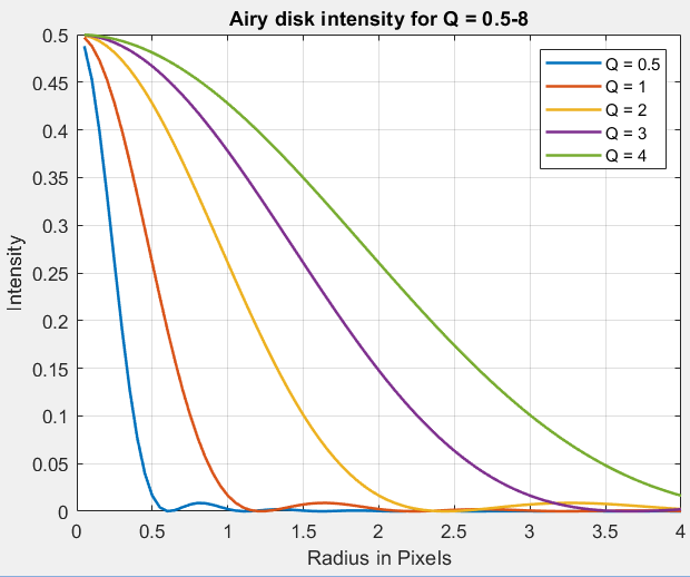 Image Modified Image Modified | 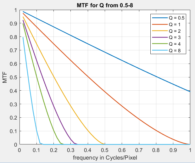 Image Modified Image Modified |
Defocus
Defocus (or misfocus or focus error) blurs the image — taking a bite out of MTF. Defocus is a large subject that we can only touch on.
...
The first step is to determine the circle of confusion diameter c for the camera at the specified test distance. Using Wikipedia's notation, where f = focal length, A = Aperture diameter, N = f-number = f/A, and S1 = lens-to-object distance,
| Eazy math inline |
|---|
| body | \displaystyle c = \frac{fA}{S_1 - f} = \frac{f^2}{N(S_1-f)} |
|---|
|
Example: an aerial camera with a pixel pitch of 3.76μm (0.00376mm) has a 110mm f/4 lens focused at infinity. We would like to know if it can be reliably tested at 100 meters. Using units of mm,
c = 1102 / (4*(100000-110)) = 12100/(4*99890) = .0303mm = 30.3μm = 8.05 pixels.
This seems large, but we need to relate this to MTF degradation to determine how bad 100 meters is.
...
For a circle of confusion with diameter c, and spatial frequency ν (in compatible units to c, i.e., pixels and cycles/pixel)
| Eazy math inline |
|---|
| body | \displaystyle OTF= 2J_1(\pi c \nu)/(\pi c \nu) |
|---|
|
,where J1 is a Bessel function of the first type, easily evaluated with the MATLAB besselj function. There is also a useful approximation:
J1 ≅ sin(0.84 πcν)/(0.84 πcν) up to the first null (0.84 πcν < π).
MTF vs spatial frequency in cycles/pixel for several values of c is shown on the right, which requires some interpretation. Typical high quality lenses have MTF50 around 0.3 cycles/pixel (this is very approximate), with MTF roughly 10-30% at the Nyquist frequency (fNyq = 0.5 C/P). MTF50 below 0.15 indicates an inferior (or misfocused) lens. MTF at Nyquist > 0.4 may be a little too sharp for the system: there can be significant aliasing effects and lens is probably more expensive than needed. With this knowledge we can say that
...
To find the distance S1 for a specified circle of confusion c, the above equation must be inverted.
| Eazy math inline |
|---|
| body | \displaystyle S_1 = f + \frac{f^2}{Nc} |
|---|
|
Example: for the above camera, if we want to find the distance for c = 2 pixels = 7.52μm = 0.00752mm,
...
OTF for combined diffraction and misfocus — can be found on page 10 of the Jacobson lens tutorial. It's a complicated equation (and not the product of the OTFs for diffraction and misfocus). For ν = spatial frequency = fsp, s = λNν, and a = πνc, where units are consistent (i.e., fsp = ν in cycles/mm for λ and c in mm).
| Eazy math inline |
|---|
| body | \displaystyle OTF = \frac{4}{\pi a} \int_{y=0}^{y=\sqrt{1-s^2}} \sin\left(a \sqrt{1-y^2}-s\right)dy, \ \ \ \ s < 1 |
|---|
|
| Eazy math inline |
|---|
| body | \displaystyle = 0; \ \ \ \ \ \text{otherwise} |
|---|
|
A result for a small aperture is shown in the tutorial.