...
This setting uses the measured of contrast of flat areas P1 and P2 (light and dark portions of each individual slanted-edge Region of Interest (ROI), away from the edge itself) to calculate the gamma for each edge. It is easy to use and quite robust. The only requirement is that the printed chart contrast ratio be known and entered. (It is 4:1 or 10:1 for nearly all Imatest slanted-edge charts.) This method is not reliable for chart contrasts higher than 10:1.
| Eazy math inline | ||
|---|---|---|
|
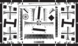
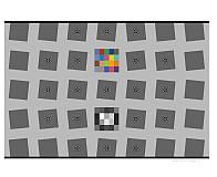
A brief history of chart contrast The ISO 12233:2000 standard called for a chart contrast of at least 50:1. This turned out to be a poor choice: The high contrast made it difficult to avoid clipping (flattening of the tonal response curve for either the lightest or darkest areas), which exaggerates MTF measurements (making them look better than reality). There is no way to calculate gamma from the ISO 12233:2000 chart (shown on the right). This issue was finally corrected with ISO 12233:2014 (later revisions are relatively minor), which specifies a 4:1 edge contrast, which not only reduces the likelihood of clipping, but also makes the MTF calculation less sensitive to the value of gamma used for linearization. The old ISO 12233:2000 chart is still widely used: we don’t recommend it. The SFRplus chart, which was introduced in 2009, originally had an edge contrast of 10:1 (often with a small number of 2:1 edges). After 2014 the standard contrast was changed to 4:1 (shown on the right). The eSFR ISO chart (derived from the 2014 standard) always has 4:1 edge contrast. Both SFRplus and eSFR ISO have grayscales for calculating tonal response and gamma. SFRreg and Checkerboard charts are available in 10:1 and 4:1 contrast. Advantages of the new charts are detailed here and here. Imatest chrome-on-glass (CoG) charts have a 10:1 contrast ratio: the lowest that can be manufactured with CoG technology. Most other CoG charts have very high contrast (1000:1, and not well-controlled). We don’t recommend them. We can produce custom CoG charts quickly if needed. |
...
We ran an image from a compact digital camera, converted from raw with dcraw, with a number of different gamma settings to see how the settings affected MTF rsults.
Tonal response from grayscale. gamma = 0.369 The chart and images are several years old. The chart may have been printed with lower contrast than intended, resulting in a lower gamma measurement. This has no effect on the relative measurements below. |
Gamma | MTF50 (C/P) | MTF Area PkNorm (C/P) |
0.20 | 0.2415 | 0.261 |
0.30 | 0.2408 | 0.258 |
0.322 | 0.2368 | 0.254 |
0.40 | 0.2387 | 0.254 |
0.50 | 0.2344 | 0.247 |
0.60 | 0.2332 | 0.247 |
\Note that errors in estimating gamma (differences from 0.322) have very little effect on MTF measurements. MTF50 and MTF Area change very slightly, even with relatively large gamma errors. This is a good place discuss Imatest’s ISO 12233 compliance. Imatest uses a simple first-order inverse of the OECF curve (tonal response) measurement to linearize the image. It does not use a higher-order inverse. But because MTF is relatively insensitive to gamma (the slope of the tonal response curve), the simple fit results in nearly identical MTF measurements (except the the exposure is close to saturation, which where it’s hard to avoid dodgy results).
...
JPEGs, on the other hand, frequently have a “shoulder”— a region where gamma (contrast) is gradually reduced— in the highlights. The shoulder improves the perceived pictorial quality of the image by reducing saturation (or “burnout”) of the highlights. It was a part of film response curves, long taken for granted. In order to achieve this shoulder, the exposure has to be reduced below the optimum level for a straight gamma curve to allow some “headroom” for the shoulder (before highlights are saturated). Here is an example: in-camera JPEG and LibRaw-converted raw images of the Colorchecker charts and doll, whose tonal response curve are shown above or the in-camera JPEG and below for the LibRaw-converted TIFF.
Here is the (nearly) straight-line density response for the converted CR2 raw image on the right. Though this image is typical, we have seen much larger differences between JPEG and converted raw files.
...
The Weber contrast
| Eazy math inline | ||
|---|---|---|
|
| Eazy math inline | ||
|---|---|---|
|
Michelson
Michelson contrast
| Eazy math inline | ||
|---|---|---|
|
| Eazy math inline | ||
|---|---|---|
|
Michelson contrast is sometimes called “modulation”, and is the basis of Modulation Transfer Function (MTF) measurements. In the SPIE Optipedia page on Modulation Transfer Function, M in equation (1.12) is none other than Michelson contrast. MTF is defined as Michelson contrast at spatial frequency f, normalized to 1 at f = 0. Amax and Amin are derived from sine waves. If sine waves are unavailable (e.g., for slanted-edges), f can be calculated from a Fourier transform (it’s 1/f for a one-dimensional edge, which has the lovely property of spatial invariance).
...
Dynamic range limitation — An issue with logarithmic spaces is that their dynamic range is strictly limited by the math since log(0) = -∞. Using the above equation and assuming that log represents log10 and n2 = 1,
| Eazy math inline | ||
|---|---|---|
|
If we assume that exp is normalized to a maximum value of expmax = 1, p(expmax) = p(1) = 1. The darkest level that can be reproduced is p(expmin) = γ log10(expmin)+1 = 0.
| Eazy math inline | ||
|---|---|---|
|
...
For gamma = 0.5 (shown in the plot, above right), expmin = 10-2 = 0.01, equivalent to
...
This brings us to the big question: Why is logarithmic encoding widely used in video/cinema systems? Coming from still photography, where gamma encoding is widely used (but log encoding isn’t), we are aware that gamma encoding accomplishes the same goals without the dynamic range limitation. If you have a good answer, please let us know. |
Misinformation warning — The Internet is full of misinformation about logarithmic color spaces. A good example is the B&H page, Understanding Log-Format Recording, which says, ” If your video—like most video—is not recorded using a log picture profile, chances are the exposure is being recorded in a linear fashion.” This is completely incorrect. The author seems to have no inkling that gamma encoding exists. Then he compounds the confusion with statements like “The problem arises with the realization that the exposure values with which we measure light are not linear. An exposure “stop” represents a doubling or halving of the actual light level, not an increase by some arbitrary linear value on a scale. You could, in fact, say exposure values are themselves logarithmic!”. Exposure Value (EV) is a relative measurement unit based on factors 2 (log2(exposure level)) that corresponds to the sensitivity of the human eye. It has nothing to do with the camera itself. For the record: Most digital sensors have a linear response, with more than 8 bits for high quality cameras (12, 14, or more bits are common). Following Analog-to-Digital conversion, most still cameras encode the image using a gamma curve. Video cameras use either gamma or log curves. As we mentioned above, this extends the effective dynamic range for gamma encoding. |
...
Parameter | Definition | ||||||||||||||||||||
Tonal response curve | The pixel response of a camera as a function of exposure. Usually expressed graphically as log pixel level vs. log exposure. | ||||||||||||||||||||
Gamma | Gamma is the average slope of log pixel levels as a function of log exposure for light through dark gray tones). For MTF calculations It is used to linearize the input data, i.e., to remove the gamma encoding applied by image processing so that MTF can be correctly calculated (using a Fourier transformation for slanted-edges, which requires a linear signal). Gamma defaults to 0.5 = 1/2, which is typical of digital camera color spaces, but may be affected by image processing (including camera or RAW converter settings) and by flare light. Small errors in gamma have little effect on MTF measurements (a 10% error in gamma results in a 2.5% error in MTF50 for a normal contrast targetfor 4:1 (low) contrast ratio edges (See How strongly does gamma affect MTF? above). Gamma should be set to 0.45 or 0.5 when dcraw or LibRaw is used to convert RAW images into sRGB or a gamma=2.2 (Adobe RGB) color space. It is typically around 1 for converted raw images that haven’t had a gamma curve applied. If gamma is set to less than 0.3 or greater than 0.8, the background will be changed to pink to indicate an unusual (possibly erroneous) selection. If the chart contrast is known and is ≤10:1 (medium or low contrast), you can enter the contrast in the Chart contrast (for gamma calc.) box, then check the Use for MTF (√) checkbox. Gamma will be calculated from the chart and displayed in the Edge/MTF plot. If chart contrast is not known you should measure gamma from a grayscale stepchart image. A grayscale is included in SFRplus, eSFR ISO and SFRreg Center ([ct]) charts. Gamma is calculated and displayed in the Tonal Response, Gamma/White Bal plot for these modules. Gamma can also be calculated from any grayscale stepchart by running Color/Tone Interactive, Color/Tone Auto, Colorcheck, or Stepchart. [A nominal value of gamma should be entered, even if the value of gamma derived from the chart (described above) is used to calculate MTF.] Gamma is the exponent of the equation that relates image file pixel level to luminance. For a monitor or print,
When the raw output of the image sensor, which is typically linear, is converted to image file pixels for a standard color space, the approximate inverse of the above operation is applied.
This is equation is an approximation because the tonal response curve (which often has a “shoulder”— a region of decreased contrast in the highlights) doesn’t follow the gamma equation exactly. It is often a good approximation for light to dark gray tones: good enough for to reliably linearize the chart image if the edge contrast isn’t too high (4:1 is recommended in the ISO 12233:2014+ standard).
In practice, gamma is equivalent to contrast. When the Use for MTF checkbox (to the right of the Chart contrast dropdown menu) is checked, camera gamma is estimated from the ratio of the light and dark pixel levels P1 and P2 in the slanted-edge region (away from the edge) if the chart contrast ratio (light/dark reflectivity) has been entered (and is 10:1 or less). Starting with
| ||||||||||||||||||||
Shoulder | A region of the tonal response near the highlights where the slope may roll off (be reduced) in order to avoid saturating (“bunring out”) highlights. Frequently found in pictorial images. Less common in machine vision images (medical, etc.) When a strong shoulder is present, the meaning of gamma is not clear. |
| Eazy math inline | ||
|---|---|---|
|


